The Mandelbrot Set as a Modular Form
Linas Vepstas <linas@linas.org>
2 January 2005 (revised 30 May 2005)
Abstract:
An exploration of the interior or the Mandelbrot Set and the appearance
of functions appearing to be similar to modular forms. This provides
yet another example of the close interconnection between the structure
of the Modular Group SL(2,Z) and fractals. The relationship is demonstrated
computationally and visually, and not from first principles; visually,
the interior resembles the Weierstrass elliptic invariant

.
However, it is a resemblance only; the various explicit expressions
that can be found are shown to not actually be modular forms. It is
hypothesized that some simple but currently unknown transformation
will convert them into modular forms.
The construction of the interior is based on averaging together iterated
values with a spectral-type summation, and then analyzing the asymptotic
behavior of the sum. Leading divergence are easy to explain and remove;
the remaining finite parts hint at modular symmetry.
This is a work in progress. A final conclusion and analysis has not
been reached.
This paper is part of a set of chapters that explore the relationship
between the real numbers, the modular group, and fractals. Updated
and revised versions of this monograph can be found at http://www.linas.org/math/sl2z.html
XXX This paper may be subject to occasional revision. XXX
Modular forms are a particular kind of function on the complex upper
half-plane studied in analytic number theory and the theory of elliptic
curves. A precise definition of a modular form[WMF] will be
given later in this paper. As a simple example, consider the Euler
function
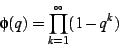 |
(1) |
on the complex plane. It is closely related to the Dedekind eta function,
which is a modular form. Figure ![[*]](/usr/share/latex2html/icons/crossref.png) shows
shows  inside the unit disk
  . Graphs of most modular forms visually
resemble this picture in one way or another. The exploration presented
in this monograph will be mostly visual, not algebraic; none-the-less,
various basic expressions will be developed to make the hypothesis
as explicit as possible.
. Graphs of most modular forms visually
resemble this picture in one way or another. The exploration presented
in this monograph will be mostly visual, not algebraic; none-the-less,
various basic expressions will be developed to make the hypothesis
as explicit as possible.
Figure:
Euler Function
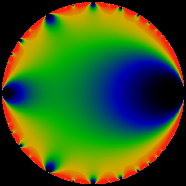
A rendition of the absolute value  of the Euler function
on the of the Euler function
on the  -disk. Note the readily apparent fractal self-similarity.
This type of self-similarity is explicitly associated with the properties
of the modular group -disk. Note the readily apparent fractal self-similarity.
This type of self-similarity is explicitly associated with the properties
of the modular group
 . A crude general resemblance
to the structure of the Mandelbrot set should be equally evident.
This paper is devoted to making this vague resemblance into a relationship
as concrete as possible. . A crude general resemblance
to the structure of the Mandelbrot set should be equally evident.
This paper is devoted to making this vague resemblance into a relationship
as concrete as possible. |
Now consider the Mandelbrot set. By means of a sequence of figures
below, we shall uncover a structure inside the Mandelbrot set that
appears to be some kind of modular form. The general development will
be as follows: the first section develops a set of series that capture
the asymptotic behavior of an iterated function. In the next section,
these series are then applied to the Mandelbrot set iterator, where
they are found to contain divergent and finite terms. The next section
develops explicit, exact expressions for the divergent terms. The
remainder of the paper is devoted to an exploration of the finite
terms, and attempts to draw analogies to such modular forms as the
Weierstrass elliptic invariant and to series involving the
divisor function. Both the main cardioid and the large western bulb
are explored. The paper concludes with an appendix reviewing the numeric
techniques of series acceleration.
This paper is an expansion and revision of an earlier paper posted
at http://www.linas.org/art-gallery/spectral/spectral.html.
This section reviews the construction of a regulated series. These
series will be used to perform a kind of averaging over the values
of an iterated function; the asymptotic behavior of an iterated function
may be studied in terms of these series.
Consider the sequence
 . Then for small
positive
. Then for small
positive  , construct the sum
 |
(2) |
In the following,we'll refer to this as the regulated series
for the sequence  . For large class of reasonably behaved
series , this sum is finite for all positive values of
. By 'reasonably behaved' we mean a sequence where
. For large class of reasonably behaved
series , this sum is finite for all positive values of
. By 'reasonably behaved' we mean a sequence where  doesn't
get exponentially large with increasing
doesn't
get exponentially large with increasing  ; that is, one where the
sum converges.
; that is, one where the
sum converges.
This sum participates in some interesting number-theoretic relationships
when the are considered to be the spectrum of an operator.
In the following, we will be considering the not as
a spectrum, but instead as the iterates of the Mandelbrot Set. Before
doing so, lets quickly review some basic properties.
One can define a Dirichlet series
 |
(3) |
which can be easily converted into the first sum with an integral
transform.
The spectral analysis consists of exploring the behavior of the sum
in the limit of  . Depending on the series, it may
diverge. For example, if we take all to be one, the sum
. Depending on the series, it may
diverge. For example, if we take all to be one, the sum
 diverges as 1/t, while
 diverges
as
diverges
as  . The corresponding Dirichlet series exhibit poles at
 and
and  , respectively, for these sums. The core idea behind
spectral analysis is that in general, one can gain insight into the
structure of the series by understanding the analytic
structure of the related series. In other words, instead of studying
directly, we study the expansion
, respectively, for these sums. The core idea behind
spectral analysis is that in general, one can gain insight into the
structure of the series by understanding the analytic
structure of the related series. In other words, instead of studying
directly, we study the expansion
 |
(4) |
instead.
When engaging in numerical calculations, the Dirichlet series is nearly
numerically intractable, because of its painfully slow convergence.
Thus,one is instantly motivated to use the exponential series instead.
However, one gets an even more stable and numerically well-behaved
series by considering the Gaussian regulator, namely
 |
(5) |
There is no harm in using this series for numerical work; it can
be related back to the Dirichlet series through analytic integral
transforms, albeit somewhat more complex ones than the plain exponential
series. This, and some numerical subtleties, are discussed in a later
section.
Now consider the standard Mandelbrot set iteration
 |
(6) |
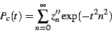
ant the regulated series for this sequence of points
 |
(7) |
where we've added the subscript  to remind us that this series
takes on distinct values for every point
to remind us that this series
takes on distinct values for every point
 . For most
of the interior of the Mandelbrot set, this sum diverges as
. For most
of the interior of the Mandelbrot set, this sum diverges as  .
To normalize this sum, let us define
.
To normalize this sum, let us define
 |
(8) |
which also diverges as . Figure shows
the nature of the divergence by normalizing against this value. As
a practical matter when performing numerical computations, it is more
appropriate to let  stand in the place of divergences, rather
than to try to use directly. The utility of this procedure
is discussed in detail in a later section on numerical methods.
stand in the place of divergences, rather
than to try to use directly. The utility of this procedure
is discussed in detail in a later section on numerical methods.
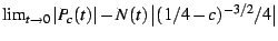
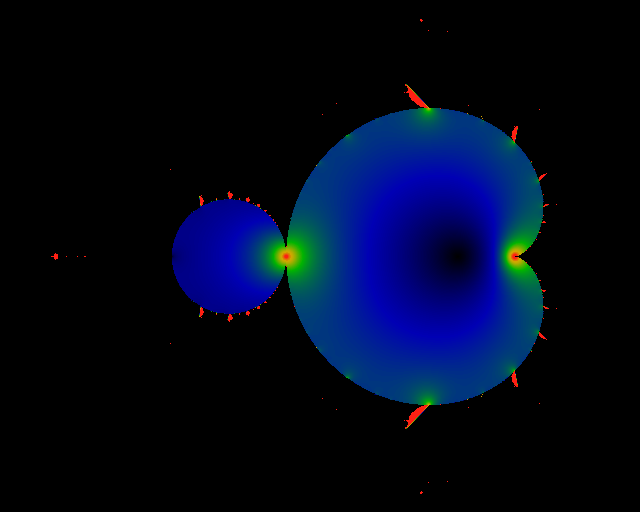
Figure:
Divergent term
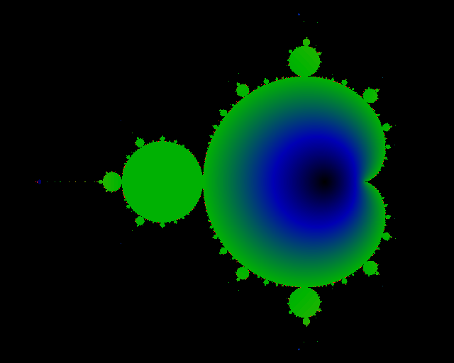
Plot of the divergent term of  . The figure shows . The figure shows
 ,
where ,
where
 is the ordinary complex
modulus. Black represents a value of zero, and green a value of 1/2.
Points outside of the M-set are explicitly excluded from this picture.
An explicit expression for this divergent term is given in the text. is the ordinary complex
modulus. Black represents a value of zero, and green a value of 1/2.
Points outside of the M-set are explicitly excluded from this picture.
An explicit expression for this divergent term is given in the text. |
The first order of business is to provide an explicit expression for
the divergent term. We can do this by considering a related and somewhat
more interesting sum, the sum over second derivatives of  with respect to . Realizing that each is parameterized
by , we can take its derivative:
with respect to . Realizing that each is parameterized
by , we can take its derivative:
 |
(9) |
and
 |
(10) |
Note that ,  and
and  are well defined for
all values of and finite : they are entire functions, 'merely'
polynomials in . Note that these polynomials never involve
are well defined for
all values of and finite : they are entire functions, 'merely'
polynomials in . Note that these polynomials never involve  ,
the complex conjugate of , and thus all derivatives with respect
to are vanishing.
,
the complex conjugate of , and thus all derivatives with respect
to are vanishing.
Let us then define the sum
 |
(11) |
Note that
 |
(12) |
holds for all positive .  also diverges as .
Figures and
shows the magnitude and phase of that divergence. By comparing the
figures, it is relatively straightforward to determine that inside
of the main cardiod, the divergent term of is given by
also diverges as .
Figures and
shows the magnitude and phase of that divergence. By comparing the
figures, it is relatively straightforward to determine that inside
of the main cardiod, the divergent term of is given by
 |
(13) |
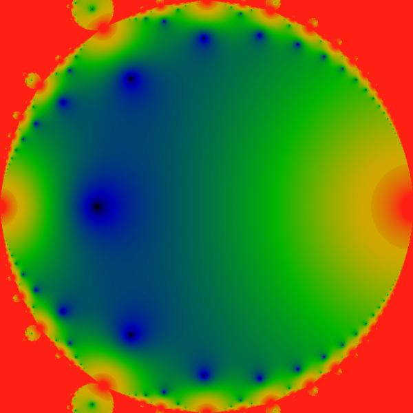
Figure:
Divergent Derivative
This picture shows the divergent term of , that is,
 .
Red denotes any value equal or greater than 1, black corresponds to
a value of zero. The value of this limit in the largest bud to the
left is precisely zero over the entire bud. For the next smallest
buds (at the top, bottom, and the second to the left), the value seems
to be uniformly 1/30 across the whole bud, although there does seem
to be a slight gradation which is hard to distinguish from numerical
errors. By looking at this image, we can see that this limit seems
to take on other, constant, values in the progressively smaller buds.
The color scheme here has black <= 0.0, blue ~= 0.2,
green ~= 0.5, yellow ~= 0.75, red
>= 1.0. If the values were indeed constant over the smaller buds,
this would have some interesting implications on the limit-cycles
for these buds, as discussed in the text. .
Red denotes any value equal or greater than 1, black corresponds to
a value of zero. The value of this limit in the largest bud to the
left is precisely zero over the entire bud. For the next smallest
buds (at the top, bottom, and the second to the left), the value seems
to be uniformly 1/30 across the whole bud, although there does seem
to be a slight gradation which is hard to distinguish from numerical
errors. By looking at this image, we can see that this limit seems
to take on other, constant, values in the progressively smaller buds.
The color scheme here has black <= 0.0, blue ~= 0.2,
green ~= 0.5, yellow ~= 0.75, red
>= 1.0. If the values were indeed constant over the smaller buds,
this would have some interesting implications on the limit-cycles
for these buds, as discussed in the text. |
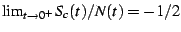
The divergent term term of can be immediately integrated
to obtain the divergent term in inside the cardiod:
![\begin{displaymath}
S_{c}(t)=N(t)\;\left[\frac{1}{2}-\sqrt{\frac{1}{4}-c}\;\right]+\mathcal{O}(1)
\end{displaymath}](img47.png) |
(14) |
If we write this divergent piece as
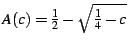 then it is trivial to verify that
 on the
boundary of the cardioid; that is,
on the
boundary of the cardioid; that is,
 for all angles
  . The boundary of the cardioid is given by
 ,
of course. Next, we note that
,
of course. Next, we note that  represents a fixed-point of
the Mandelbrot iterator:
represents a fixed-point of
the Mandelbrot iterator:
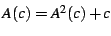 . Indeed, this should not
be a surprise: the divergent term of the sum is in effect
the average over over all values of . Inside the main bulb,
we have
. Indeed, this should not
be a surprise: the divergent term of the sum is in effect
the average over over all values of . Inside the main bulb,
we have
 , and so of necessity,
the leading divergence of the sum must be . Similarly, in the
large bud on the left, converges to a two-cycle, with
, and so of necessity,
the leading divergence of the sum must be . Similarly, in the
large bud on the left, converges to a two-cycle, with
 and
and
 . The average of these
two values is
. The average of these
two values is  , and so we can trivially deduce that
 and thus that
 which exactly matches our numerical results. In other buds, the sequence
converges to m-cycles. Thus, in other buds, the divergent term will
be the average over these m values of the limit cycle. Provided one
can calculate this average, then one has an exact expression for the
divergences of . Of course, there are considerable additional
difficulties once one gets into the more contorted parts of the M-set,
since the convergence to a limit cycle can be extremely slow, thus
creating considerable topological difficulties when reasoning about
the topology of the M-set and in particular, the validity of the expansion
of terms in the formula . The remainder of
this monograph concerns itself with the issue of the rate of convergence
to the limit cycles, which we will find is given by the Dedekind eta.
which exactly matches our numerical results. In other buds, the sequence
converges to m-cycles. Thus, in other buds, the divergent term will
be the average over these m values of the limit cycle. Provided one
can calculate this average, then one has an exact expression for the
divergences of . Of course, there are considerable additional
difficulties once one gets into the more contorted parts of the M-set,
since the convergence to a limit cycle can be extremely slow, thus
creating considerable topological difficulties when reasoning about
the topology of the M-set and in particular, the validity of the expansion
of terms in the formula . The remainder of
this monograph concerns itself with the issue of the rate of convergence
to the limit cycles, which we will find is given by the Dedekind eta.
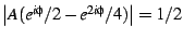
Let us now turn to the finite remainders. By subtracting away the
divergent pieces, we are essentially subtracting away the contribution
of the asymptotic limit cycle. The remaining finite parts indicate
how the asymptotic behavior is approached. If the finite part is large,
this indicates that the iteration took a long time to approach the
asymptotic limit. If the finite part is small, then the series converged
to its limit cycle quickly. The figure
shows this rate of convergence. Curiously, we find that
 |
(15) |
that is, the divergence of the modulus has the opposite sign from
the divergence of the sum. This can only happen if the phase (the
argument) of the finite part is opposite to the phase of .
In other words,
 |
(16) |
The overall structure at first doesn't look all that inspiring. As
before, we can discern considerably more structure if we examine
instead of . This reveals some of the true complexity in
the system.
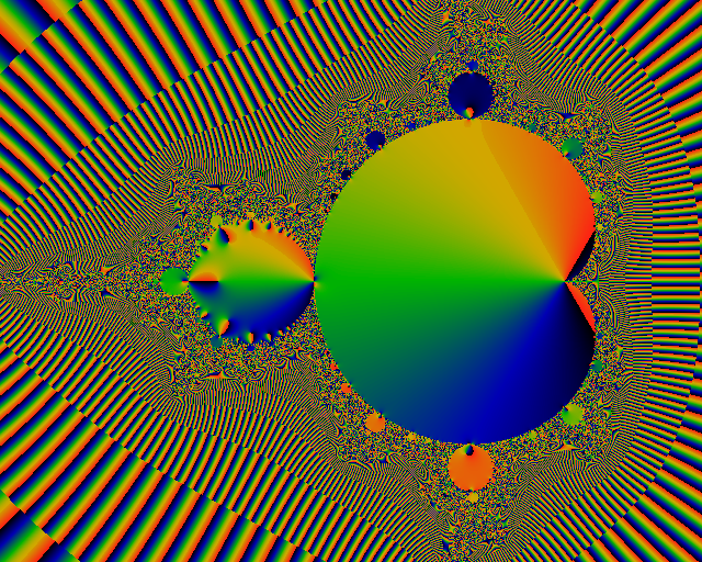
The finite term in the main cardiod is shown in figure
and at least a superficial resemblance to the image of the Dedekind
zeta/Euler function shown in figure should
be immediately apparent.
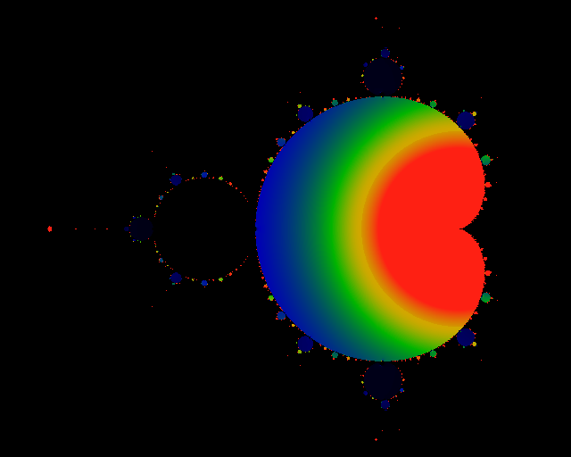
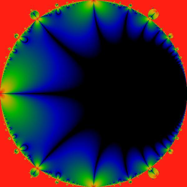
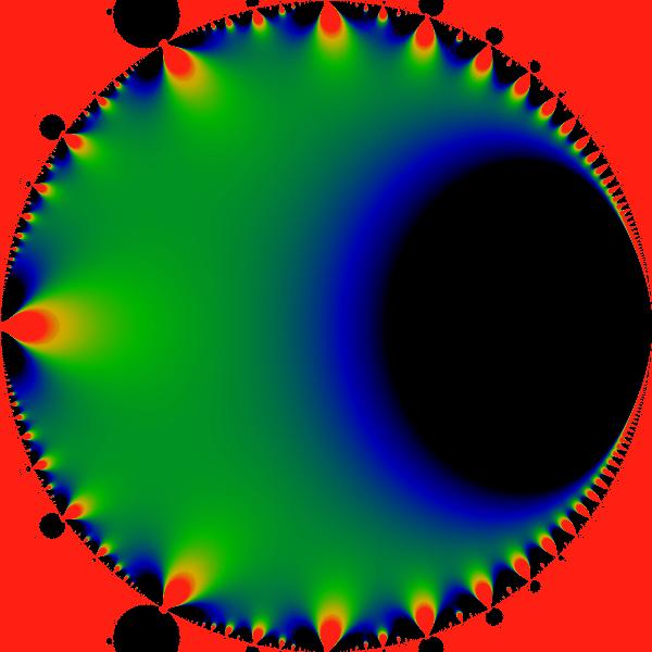
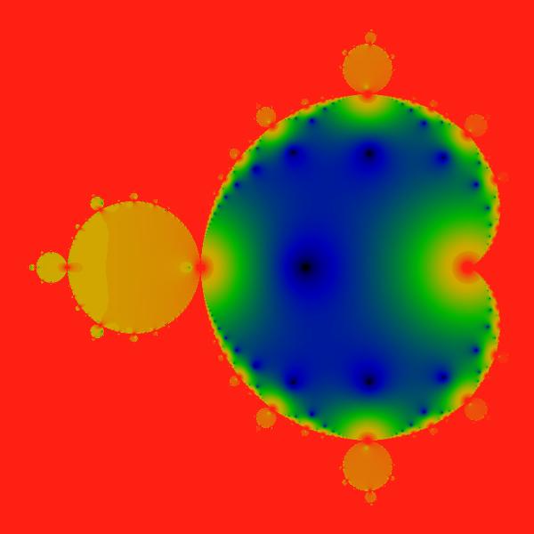
Figure:
Mandelbrot Interior
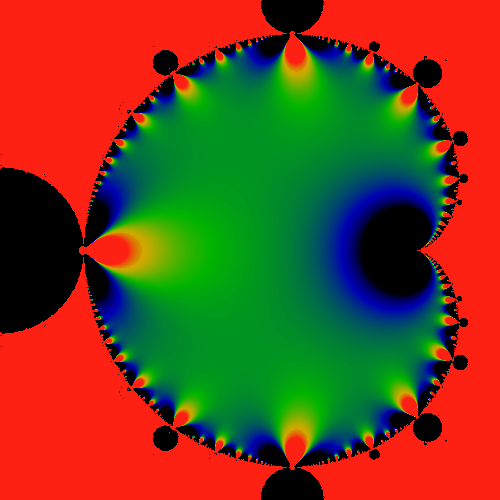
The image above shows the finite piece in the main bulb, after the
divergent piece has been subtracted. That is, it shows
 .
It appears to have dipoles (saddles) arrayed along the perimeter.
There don't seem to be any simple zeros. The color scheme has been
adjusted so that black <= -10, green ~= 0 and red
>= 10. These (multi-)poles visually indicate something that is commonly
known: the series has a hard time converging near the tips of the
horns. .
It appears to have dipoles (saddles) arrayed along the perimeter.
There don't seem to be any simple zeros. The color scheme has been
adjusted so that black <= -10, green ~= 0 and red
>= 10. These (multi-)poles visually indicate something that is commonly
known: the series has a hard time converging near the tips of the
horns. |
It is important at this point to note that this last figure shows
the modulus taken first, and then the divergence subtracted afterwards.
This is not the same as subtracting the divergence first, and then
taking the modulus. If we subtract the divergent complex term first,
then we see in the main cardiod a figure that closely resembles that
in figure , with a complex structure of poles
located on the boundary, and zeros located inside.
The sums on the main circular bud immediately to the west of the cardioid
do not have a divergent parts; the sums appear to be finite. The bud
interior is shown in the figure .
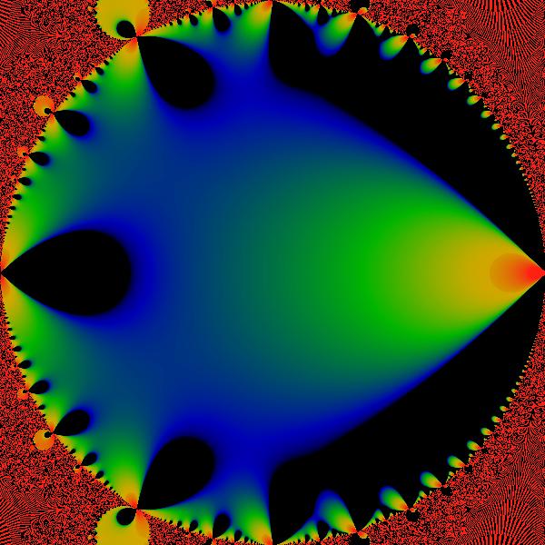
Figure:
Bud Interior
The sum doesn't have a divergent piece in the large bud.
This image shows
 for the square area
![$\Re c\in[-1.25,-0.75]$](img66.png) . As can be seen, there
is a considerable amount of structure here. There seem to be poles
located on the boundary, where-ever another bud is tangent to this
one. This is of course everywhere, since a bud is tangent for every
possible rational angle. The strength of the pole is somehow proportionate
to the size of the bud; the residue of the poles all seem to be the
same sign. Note there seems to be a sequences of zeros inside the
bud. The color ramp has been logarithmically compressed to highlight
the zeros: black = 0, green ~= 10, red >= 100. . As can be seen, there
is a considerable amount of structure here. There seem to be poles
located on the boundary, where-ever another bud is tangent to this
one. This is of course everywhere, since a bud is tangent for every
possible rational angle. The strength of the pole is somehow proportionate
to the size of the bud; the residue of the poles all seem to be the
same sign. Note there seems to be a sequences of zeros inside the
bud. The color ramp has been logarithmically compressed to highlight
the zeros: black = 0, green ~= 10, red >= 100.
A very similar figure results if one graphs the finite part on the
main cardiod, after removing the divergence. That is, the graph for
 in the main cardiod is essentially the same.
 |
The bud interior shows a remarkable visual resemblance to the divisor
series
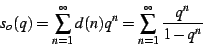 |
(17) |
constructed from the classic number-theoretic divisor function
 ,
the number of divisors of . Figure shows
the divisor series.
,
the number of divisors of . Figure shows
the divisor series.
Figure:
Divisor Series on the q-disk
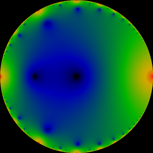
The sum
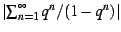 on the
unit disk. The colormap is logarithmically compressed, so that blue
represents ares with a value of less than one, and green represents
areas with a value of more than 10. on the
unit disk. The colormap is logarithmically compressed, so that blue
represents ares with a value of less than one, and green represents
areas with a value of more than 10. |
Re-expressing the coordinates on the interior of the bud as
 |
(18) |
so that the center of the bud occurs at  and the radius of
the bud is
and the radius of
the bud is  , one can then produce a rough numeric fit to the
q-series for the interior of the bud. It seems that
, one can then produce a rough numeric fit to the
q-series for the interior of the bud. It seems that
 |
(19) |
The numbers in parenthesis give the uncertainty in the least significant
digit. This is a fairly quick and rough fit; only the values of the
first two terms seem certain, and that the coefficient of  seems to vanish.
Figure shows the real part of  in
the bud.
in
the bud.
Figure:
Real Part
This figure shows the real part of
 in the western bud. The color scheme is identical to that used to
show the modulus. Black areas here represent negative values for the
real part. A similar graph of the divisor series would have more or
less a rather similar look.
in the western bud. The color scheme is identical to that used to
show the modulus. Black areas here represent negative values for the
real part. A similar graph of the divisor series would have more or
less a rather similar look. |
Explicit numerical work shows that it does not seem to be a modular
form of integer weight. Nor does it seem to be a modular form of fractional
weight. But it sure seems to ``come close''. Lets review what
this means.
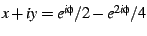
Modular symmetry on the -disk is best explored by mapping the
-disk to the Poincare upper half-plane, applying a Mobius transformation
there, and then mapping back. Given a point  in the upper half-plane,
i.e.
in the upper half-plane,
i.e.  , one maps to the -disk with
 |
(20) |
One can then apply a Mobius transform to on the upper half
plane:
 |
(21) |
and then map this back to the -disk coordinates.
A function  on the upper half-plane is said to be a modular
form if
on the upper half-plane is said to be a modular
form if
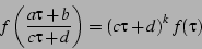 |
(22) |
for integers  satisfying
  . The constant
  is said to be the weight of the form. Mapped to the upper half-plane,
the interior of the bud does not seem to be a modular form for any
real value of . In particular, equation
doesn't quite seem to hold even if the absolute value of each side
is taken, although it seems to ``come close'' in certain situations.
is said to be the weight of the form. Mapped to the upper half-plane,
the interior of the bud does not seem to be a modular form for any
real value of . In particular, equation
doesn't quite seem to hold even if the absolute value of each side
is taken, although it seems to ``come close'' in certain situations.
There is one interesting mapping whose properties are worth reviewing,
and that is the mapping of the upper half-plane to the Poincare disk.
This mapping is curious because it is not infrequent in the literature,
and because a periodic function on the upper half-plane takes the
appearance of a self-similar function on the disk.
The mapping if the upper half-plane to the Poincare disk is given
by
 |
(23) |
This map is a conformal map that takes points in the upper half-plane
to points in the interior of a unit disk. Points on the real number
line (points with a zero imaginary component) are mapped to the edge
of the disk. Let
 and take
  ; one
then has
; one
then has
 |
(24) |
It is not hard to show that  ; that is
  is on the edge
of the disk. A function which is periodic in with integer
periodicity will manifest itself with an M-set like periodicity on
the circumference of the Poincare disk. Specifically, a feature located
at integer values of
is on the edge
of the disk. A function which is periodic in with integer
periodicity will manifest itself with an M-set like periodicity on
the circumference of the Poincare disk. Specifically, a feature located
at integer values of  will have a specific angular location
on the Poincare disk, which is obtained by solving for the angle
will have a specific angular location
on the Poincare disk, which is obtained by solving for the angle  in
in
 |
(25) |
In particular, the region
 is mapped to the
angular interval
is mapped to the
angular interval
![$[\theta_{n},\theta_{n+1}]$](img97.png) .
.
Images constructed by mapping the -disk to upper half-plane, via
equation , will be inherently periodic. The
Mobius transform
 |
(26) |
under the -disk mapping takes all such values to exactly the
same value of . An image on the Poincare disk constructed from
the image on the -disk will have regions that are identical, by
construction.
The figures and
show a mapping of the western bud to the Poincare disk. More precisely,
the mapping is actually a half-angle mapping, taking to  instead of
  , and then re-mapping to the Poincare disk.
The result of the half-angle mapping is that the figures do not have
the left-right symmetry
, and then re-mapping to the Poincare disk.
The result of the half-angle mapping is that the figures do not have
the left-right symmetry
 , but this is only an artifact
of the construction.
, but this is only an artifact
of the construction.
Figure:
Imaginary Part on Poincare Disk
This figure shows the absolute value of the imaginary part of
in the western bud, remapped by means of the half-angle mapping, onto
the Poincare disk. The color scheme is identical to that used in other
graphs. As the values shown here are by definition positive, the color
black corresponds to small but positive values. |
In order to proceed with the exploration of the interior of the Mandelbrot
set as a modular form, we need to find a way of mapping the the cardioid
to the complex upper half-plane. The most obvious mapping is to express
the interior in terms of the coordinates  and with
the interior given by
and with
the interior given by
 |
(27) |
Thus, the rectangle  and
and
 is mapped
to the interior of the cardioid. The result of this mapping is shown
in figure.
is mapped
to the interior of the cardioid. The result of this mapping is shown
in figure.
Figure:
Circularized Cardioid
The cardioid interior remapped to the circle
 .
Bulbs on the exterior of the Mandelbrot set are also visible in this
remapping. The color scheme used is identical to that of the figure
. The additional factor of .
Bulbs on the exterior of the Mandelbrot set are also visible in this
remapping. The color scheme used is identical to that of the figure
. The additional factor of  merely left-right reflects the image.
 |
The linearized coordinates can be immediately remapped to a circle
by using the coordinates
 |
(28) |
where an extra factor of  is introduced to left-right reverse
the image. This extra flip is needed to bring the coordinate system
precisely into line with the Poincare punctured disk coordinates.
The punctured disk coordinates are sometimes referred to as the ``nome''
coordinates of elliptic geometry. These are defined as follows. Let
is introduced to left-right reverse
the image. This extra flip is needed to bring the coordinate system
precisely into line with the Poincare punctured disk coordinates.
The punctured disk coordinates are sometimes referred to as the ``nome''
coordinates of elliptic geometry. These are defined as follows. Let
 be the so-called ``half-period ratio'',
where
be the so-called ``half-period ratio'',
where  and
and  are the periods of an elliptic
function, such as the Weierstrass
are the periods of an elliptic
function, such as the Weierstrass  function. Then is
a coordinate on the upper half-plane, with . The traditional
``fundamental region'' on the upper half-plane is defined as the
region
function. Then is
a coordinate on the upper half-plane, with . The traditional
``fundamental region'' on the upper half-plane is defined as the
region
 and
and  . This coordinate system
on the upper half-plane can be mapped to the punctured disk as
. This coordinate system
on the upper half-plane can be mapped to the punctured disk as
 |
(29) |
with the word ``puncture'' referring to the fact that
never occurs for finite values of . This mapping maps the upper
half-plane to values of . The orientation of this mapping
is specifically picked in order to be consistent with standard definitions
of modular functions on the punctured disk. For example, the Euler
phi-function, expressed in coordinates, is
|
(30) |
and is show in figure .
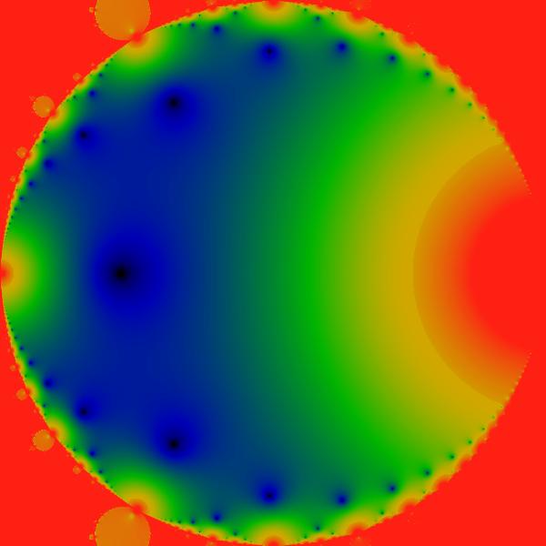
The cardioid interior should be compared to the image of the Weierstrass
invariant , shown in figure .
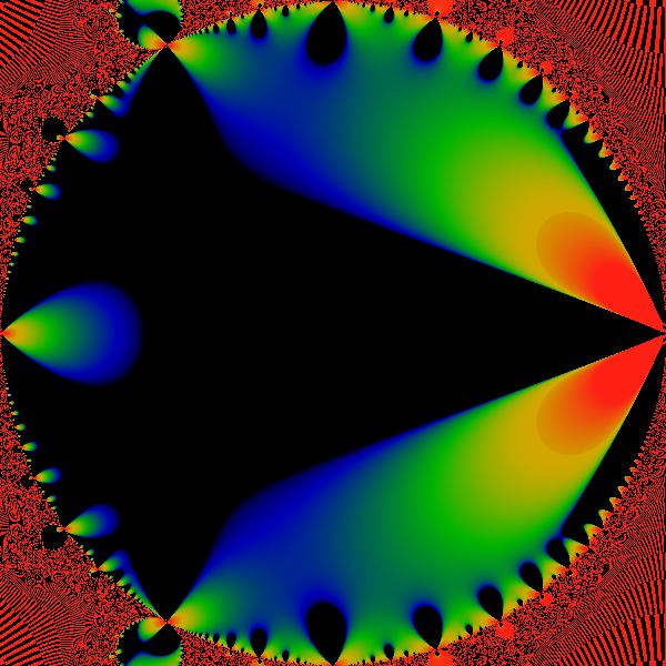
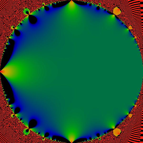
Figure:
Weierstrass invariant
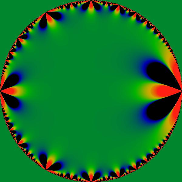
An image of the the real part of the Weierstrass invariant
expressed in coordinates. This function can be written explicitly
as
which can be re-expressed as a Lambert series
This image uses a highly compressed logarithmic color scale adjusted
to resemble that used for the Mandelbrot interior. Note that the modulus
of does not show this lobe structure; the real and imaginary
parts of this function have complementary values. Graphs of  resemble this figure, as do those of higher terms in the Eisenstein
series. As one goes up the series, the number of lobes increases arithmetically.
For example, the above figure shows three red lobes; the comparable
figure for shows four lobes.
resemble this figure, as do those of higher terms in the Eisenstein
series. As one goes up the series, the number of lobes increases arithmetically.
For example, the above figure shows three red lobes; the comparable
figure for shows four lobes. |
By comparing the figures for the interior of the Mandelbrot set and
the Weierstrass elliptic invariant, a general resemblance becomes
painfully apparent, even if not explicitly demonstrated.
By construction, the function just demonstrated on the interior of
the Mandelbrot set is a real function. To more fully explore the modular
symmetry, we really need a complex function, that is, one with real
and imaginary parts. Such a function is provided by not working with
the modulus, but subtracting the divergence directly; this is explored
in the next section.
There is also a more subtle issue. It is not clear that the simple
cardiod mapping is the correct mapping.
If one examines the figures, one can note a subtle, ever-so-slightly
visible feature. Each of the ``flames'' in the figure lean slightly
over to the right. Under Mobius transforms, this tilt is preserved,
destroying the naive symmetry. Its possible that the mapping from
cardioid to coordinates is not the right mapping, and that some
other, more complex mapping is required. What this mapping may be
is not clear at this point.
This problem is presumably related to the fact that the buds on the
exterior of the M-set are almost circles, but not quite (with the
exception of the main bud to the west). If one could find a suitable
remapping on the exterior, that mapping might presumably carry over
into the interior as well, and vice-versa.
Lets revisit, this time exploring the function
![\begin{displaymath}
\Xi(c)=\lim_{t\rightarrow0}\left[P_{c}(t)-N(t)\;\frac{\left(\frac{1}{4}-c\right)^{3/2}}{4}\right]
\end{displaymath}](img122.png) |
(31) |
Using the mappings given previously,  can be re-expressed
as
can be re-expressed
as  on the -disk. It is shown in the figures
and and .
on the -disk. It is shown in the figures
and and .
Figure:
Cardioid Finite Part
This figure shows the modulus of the finite part
 .
Some of the rest of the M-set is visible, but for the most part is
blanked out by the subtraction of the divergent term in the main cardioid.
Since this divergent term is inappropriate for the other parts of
the M-set, these other features wash out. The same compressed logarithmic
color scheme is used as in the other illustrations. .
Some of the rest of the M-set is visible, but for the most part is
blanked out by the subtraction of the divergent term in the main cardioid.
Since this divergent term is inappropriate for the other parts of
the M-set, these other features wash out. The same compressed logarithmic
color scheme is used as in the other illustrations. |
Figure:
Finite Real Part
The real part  on the -disk. The same color scheme
is used as elsewhere. on the -disk. The same color scheme
is used as elsewhere. |
Despite the remarkably suggestive graphics, it seems that  is
not a modular form either; in particular, I was unable to find a real-valued
number for which even the less-demanding relation
is
not a modular form either; in particular, I was unable to find a real-valued
number for which even the less-demanding relation
 |
(32) |
held true. (Here, the use of the symbol implies that the relation
was search for on the upper half-plane and not on the disk). It certainly
remains quite possible that minus some constant will be a modular
form, or that some further transformation of will render it
so.
This section reviews the numeric techniques applied to perform the
series sums. Specifically, some well-known techniques for series acceleration
are applied; but these are not so well known as not to merit review.
Note that the series explored on these pages can be slow to converge,
especially near the 'horns' of the Mandelbrot set. There are several
well-known and established techniques of series acceleration that
can improve the convergence. This section quickly reviews the technique
used in this paper.
Consider the sum
 |
(33) |
Assume that this sum converges in the limit of
 ,
but possibly slowly. One can get a much more quickly-converging series
by computing, in addition to
,
but possibly slowly. One can get a much more quickly-converging series
by computing, in addition to  , the derivatives
  and
and
 . One then recombines these derivatives to
form the quantity
. One then recombines these derivatives to
form the quantity
 |
(34) |
It is clear that if the limit  exists and is finite, then
one has
exists and is finite, then
one has
 |
(35) |
and furthermore, for small  one has
 |
(36) |
The correctness of equation at first seems
naively 'obvious' but is in fact quite subtle, and depends on having
a series that is 'well-behaved' in certain ways.
The study of such series and the numerical techniques to sum them
falls under the name of 'series acceleration' and is a well-developed
branch of mathematics in its own right. It is outside of the scope
of this section to review any deeper results. Suffice it to say that
this entire paper is predicated on the assumption that the equation
does hold for the sums encountered. This does
seem to be the case, but is hardly obvious from first principles,
especially for points in troublesome sections of the M-set. By contrast,
in the well-behaved areas of the M-set, it is straightforward to verify
that equation holds, and that the resulting
sums are accurate for five to ten decimal places, corresponding to
values in the range of 0.01 to 0.001 for sums with 2 to 50 thousand
terms.
Some of the sums in encountered in this paper are divergent. The simplest
such sums have a limit point, namely
 |
(37) |
in which case one has
 |
(38) |
The extra factor of  comes from the behavior of the
Gaussian regulator; that is,
comes from the behavior of the
Gaussian regulator; that is,
 |
(39) |
In order to correctly subtract this linear divergence from a divergent
sum, one is advised to subtract rather than directly.
This advice comes from the need to subtract the divergence so that
the equation is not violated. In general,
will have
 ,
,
 and
and
 terms as well, any one of which will mess up equation
if not properly accounted for. Thus, in general, the correct way to
subtract a divergent term is to form
terms as well, any one of which will mess up equation
if not properly accounted for. Thus, in general, the correct way to
subtract a divergent term is to form
 |
(40) |
and then form  from
from  to obtain the finite part. One
can perform the subtraction under the summation,
or outside of it. Performing it under the summation potentially minimizes
round-off errors. Note that these considerations apply to series with
limit cycles as well as limit points. That is, the need not
converge to a point; as long as they do converge to a limit cycle,
this mechanism of subtracting the divergent piece will work.
to obtain the finite part. One
can perform the subtraction under the summation,
or outside of it. Performing it under the summation potentially minimizes
round-off errors. Note that these considerations apply to series with
limit cycles as well as limit points. That is, the need not
converge to a point; as long as they do converge to a limit cycle,
this mechanism of subtracting the divergent piece will work.
One final remark: note that, in general, after removing a linear divergence
in a summation, the next leading order need not be finite, but may
be a weaker divergence, such as a logarithmic divergence. This is
presumably the nature of the divergences seen at the horns of the
M-set, for example. On the complex plane, finite sums grow until they
hit a pole. At the pole, the sums are logarithmically divergent.
This paper reprises and revises an earlier draft from November 2000,
located at http://www.linas.org/art-gallery/spectral/spectral.html.
Although an explicit expression for the apparent modular symmetry
was not found, it is believed that a convincing argument has been
made that such a symmetry lurks within the asymptotic limits of the
Mandelbrot iterator. Specifically, the actual symmetry appears to
most closely resemble that of sums involving the number-theoretic
divisor function. Obtaining an explicit form will open up additional
avenues of research, possibly shedding light on the maddening contour
of the Mandelbrot Set.
What more can we say? This is wild stuff.
- Apo90
- Tom M. Apostol, Modular Functions and Dirichlet Series in Number
Theory, Springer Verlag, New York, 1990.
- WMF
- Wikipedia, Modular forms, http://en.wikipedia.org/wiki/Modular_form
- Lin00
- Linas Vepstas, Spectral Analysis of Mandelbrot Interior, (2000)
located at http://www.linas.org/art-gallery/spectral/spectral.html.
Linas Vepstas
2005-05-30
![\begin{displaymath}
g_{2}(\tau)=\frac{4\pi^{4}}{3}\left[1+240\sum_{k=1}^{\infty}\sigma_{3}(k)q^{2k}\right]\end{displaymath}](img119.png)
![\begin{displaymath}
g_{2}(\tau)=\frac{4\pi^{4}}{3}\left[1+240\sum_{k=1}^{\infty}\frac{k^{3}q^{2k}}{1-q^{2k}}\right]\end{displaymath}](img120.png)